The theory of Astronavigation

This is the second in a series of articles on celestial navigation. It sets out the theory needed to understand how the technique works. The focus is on understanding, rather than calculation: we’re looking at the big picture. No calculations!

The idea is to understand the simplifications required to arrive at the most commonly used method for determining one’s position, namely the Marcq Saint-Hilaire method. Having a good grasp of this theory enables one to understand the recipe. In doing so, we minimise calculation errors when applying it.

Astronomical navigation developed alongside the needs of navigation and our understanding of astronomy. Its development began at a time when the Greeks believed that the Earth was at the centre of the universe (the Aristotelian model). We now know that many of the ideas used in this theory are, in the sense of Ockham’s razor, false. These ideas remain in use because they allow for functional method.

Four simplifications for a practical theory

The entire apparatus of astronomical navigation calculations is based on four simplifications. We assume:

1. that the Earth is at the centre of the universe;
2. that the stars are fixed;
3. that the stars are so far away that the rays of light emanating from them are parallel;
4. that any segment of a circle, if sufficiently small, is indistinguishable from a straight line.

A coordinate system

If we accept the first two simplifications, then the angular position of each star is fixed. This allows us to establish an angular coordinate system for mapping the positions of the stars.

We recall that a coordinate system requires a reference point and two axes with a scale. On the celestial sphere, the reference point is the intersection of the Greenwich meridian and the equator (coordinate (0°, 0°)). The two axes are called latitude and longitude and are measured in degrees.

Latitude spans the Earth’s sphere from south to north, and longitude from east to west. Thus, if someone is told to go to the position 10°N, 20°W, they must go 10° north of the equator and 20° west of the Greenwich meridian.

The Celestial Sphere

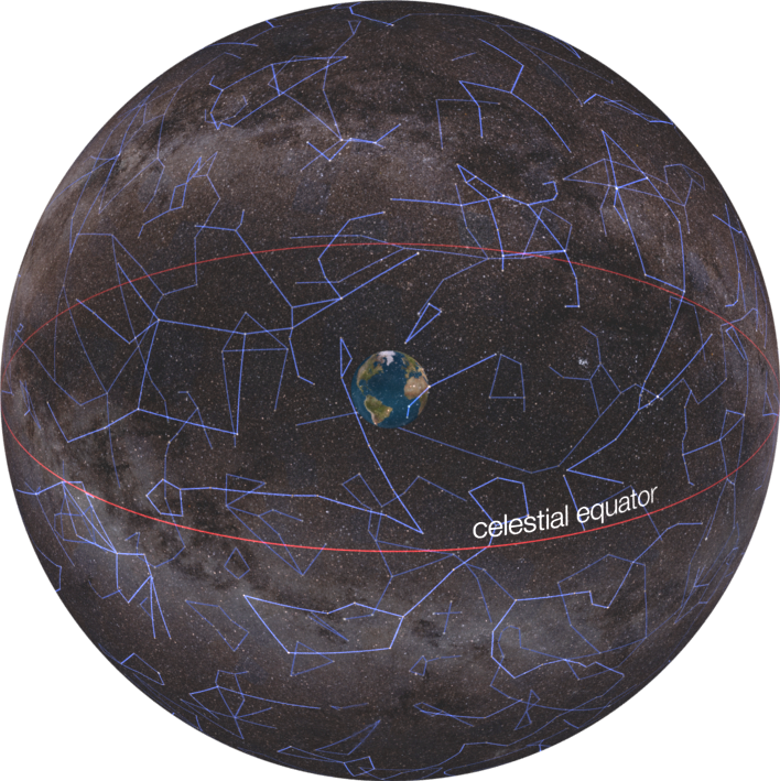
The idea is the same with the map of the universe. One must imagine a celestial sphere, where the stars are located, and that the centre of this sphere is the centre of the Earth. This sphere is infinitely large, but the stars are always at the same angles on this sphere.

On this sphere, we must establish a reference point, followed by two axes to measure positions. By convention, the reference point is called the point of Aries. In almanacs, it is sometimes denoted by the symbol for Capricorn (♈).

On this sphere, latitude and longitude are replaced by declination (Dec) and the sidereal hour angle (SHA). These terms have almost the same meaning as latitude and longitude.

Declination measures how far north or south one is on the celestial sphere. It uses exactly the same units as latitude. It ranges from 90°S to 90°N, depending on whether one is below or above the celestial equator. One simply needs to remember that one is sweeping across the celestial sphere rather than across the Earth.

The sidereal hour angle measures how far east or west one is on the sphere. However, the convention is to measure from 0° to 360° rather than from 180°E to 180°W. The sidereal hour angle thus starts at 0° at the point of aries and, as one moves westwards, the sidereal hour angle reaches 360° (a full circle). This difference in convention will lead to some complications when it comes to the calculation stages.

The table below summarises the correspondences between the two coordinate systems.

The sky chart

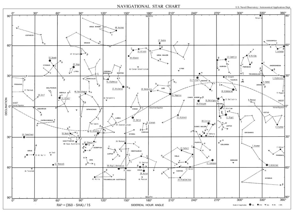
A coordinate system allows us to create a star chart using a Mercator projection. Below is a modern navigational chart produced by the US Naval Observatory. The ‘east–west’ axis is the sidereal hour angle and the ‘north–south’ axis is the declination. The vernal equinox (♈) is the point (0°, 0°) on the chart, i.e. on the left and at the centre of the image.

With such a chart, one can use the coordinate system to locate stars. For example, the star Polaris (the North Star) is approximately at the coordinates 90°N, 330°, meaning that its declination is 90° north and its sidereal hour angle is 330°. Similarly, the star Hadar is roughly at the coordinates 60°S, 150°.

E pur si mueve!

The theory of celestial navigation assumes that the stars are fixed. However, the Earth rotates at the rate of 15° per hour (360°/24 = 15° per hour). Thus, from the Earth’s perspective, the celestial sphere rotates at a rate of 15° per hour. The same applies to the point of Aries (♈): it moves with the celestial sphere.

This is a key point to understand: despite stars being fixed, earh’s rotation make it such that they rotate at a rate of 15° per hour. To position a star with earth’s coordinate, we thus need a time and a date.

This idea is directly encoded in the coordinate systems. The Sideral hour angle (SHA) of a star, whose reference point is the point of Aries, is fixed (because the point of Aries is fixed on the celestial sphere). However, the Greenwich hour angle (GHA) of a star, whose reference point is the Greenwich meridian, changes at the rate of 15° per hour. This is so because the Greenwich meridian rotates with the earth.

It is the role of almanacs to provide, for every hour and every day of the year, the position of the point of Aries relative to the Greenwich meridian. Because the relative distance between this point and each star is fixed, we can then find its GHA through calculations.

Accordingly, we can find the position of any star with terrestrial coordinates. At these coordinates, the start is directly overhead. We say that the star is at our zenith (image below).

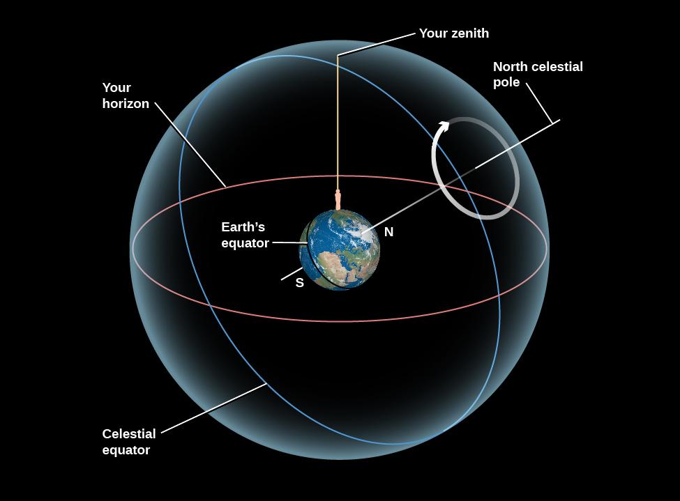
Geometrically, the terrestrial coordinate of the zenith corresponds to the point where the line connecting the star to the centre of the Earth intersects the Earth’s surface. This location is called the geographical position (GP) of the celestial body. Because the Earth rotates, the geographical position of the celestial body is constantly changing. An almanac and a star chart can therefore be used to find the geographical position of a celestial body at any time of day.

Rays of light coming from stars are parallel

The third simplification is to assume that the stars are infinitely far from the Earth. This simplification implies that the rays of light arriving from the star are, regardless of where we are on Earth, parallel. This geometric simplification allows the angle measurement taken with the sextant to be converted into a distance measurement at the GP of the celestial body. Position circles can thus be established.

The figure below illustrates this notion. It is important, and time must be taken to fully understand it. On the right of the Figure, we see the star and the rays of light going to earth (on the left). For the purpose of illustration, only two ray of lights – pictured as dashed lines – are shown. Both ray of lights are parallel. The first ray of lights hits the position of an observer on Earth. The second ray of light hits the center of the Earth. Accordingly, this second ray of light defines the GP of the star.

On the left, we see the Earth’s sphere. The position of the observer is on top, near the arrow with the word « Nous » (the French word for « us »). The angle between the observer’s horizon and the ray of light is shown in green, (labelled \theta in the Figure). This angle is precisely what a sextant measures.

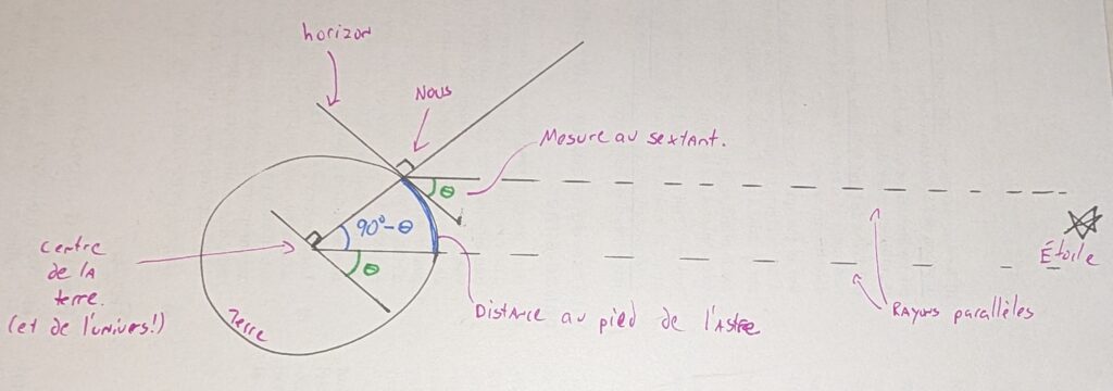
Now, let’s project this angle onto the centre of the Earth whilst keeping the horizon parallel. In the Figure, this angle is also shown in green, but at the center of the Earth. We should note that at the center of the earth, the angle between the position and the horizon is 90°. Accordingly, the angle between our position and the GP of the star is 90° - \theta (in blue in the Figure).

Recall that the definition of one nautical mile is one arcminute (one sixtieth of a degree) of earth’s circumference (1852 m). Consequently, if we take the angle 90° - \theta and multiply it by 60 arcminutes, we obtain the distance to the GP of the celestial body in nautical miles. Hence, if we see an angle \theta on the sextant, we necessarily are 60(90° - \theta) nautical miles away from the GP of the star.

The almanac tells us exactly what is the GP of a star at the moment we took our sextant sight. Accordingly, we can find a circle of position around the GP of a star whose radius is, in nautical miles, equal to 60(90° - \theta). Our ship is necessarily on this circle.

We simply need to repeat the process

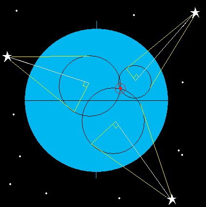
If we take several observations of celestial bodies, we then obtain several circles of position. Since we are necessarily on these circles of position, their intersection corresponds to our position. The image below summarises the idea with three celestial body measurements. The GP of each celestial body is indicated by the right-angle symbols in yellow. The circles of position are in black. The yellow radii correspond to the distance calculated by 90° - \theta. The intersection of the three circles (red dot) thus gives one and only one position: the ship’s position.

The small segments of a circle are straight lines

In principle, this is where the theory of celestial navigation ends, as we have succeeded in converting celestial measurements into a position on earth. However, a significant practical challenge remains: the position radii span distances of several hundred nautical miles, making it impossible to plot them on a chart. On a standard-sized globe (~12 inches in diameter), the intersection of the position radii would be blurred due to the scale of the globe… and due to the size of the pencils!

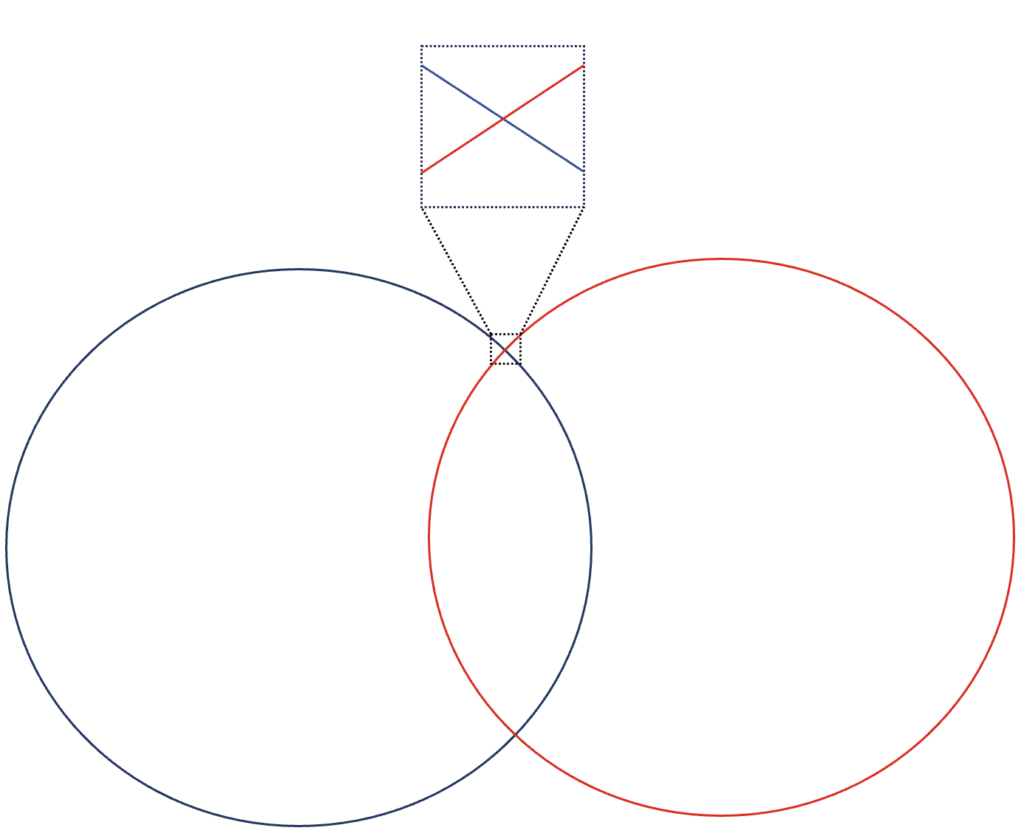
We therefore need a technique to reduce the circles of position to the scale of nautical charts. To this end, it is worth noting that with a sufficiently high resolution (zoom), any segment of a circle of position will eventually resemble a straight line. The image below summarises the idea: the two position circles, when scaled down to chart size, give the impression of two position lines (whose intersection is, of course, the position).

It is up to you whether to use the methods in publication Ho 249 or spherical trigonometry equations to convert the circles of position into line segments that can be used for plotting on a chart. This technique is the subject of an entire text.

That’s a lot of approximations!

It is clear that the simplifications used in the theory of celestial navigation generate errors. The Earth is not at the centre of the universe. But this is the valuable part of the technique: the errors are significant in conceptual terms, but have little impact on determining the position.

The stars move relative to us… and they move relative to one another. Nothing is fixed, as the theory assumes. Behind the scenes, the astronomers who compile the almanacs take stellar drift into account: this is why these publications are annual and need to be updated. The errors arising from this simplification are thus corrected over time.

The same applies to the distance to the stars: this distance is finite and measured in billions of kilometres (and more). On a planetary scale, these distances are so vast that we can say they are infinitely far apart. So even if the rays coming from the stars are not exactly parallel, they are so close to being so that the error is negligible.

In short, the theory behind celestial navigation is very similar to the mindset behind systems design in engineering: the simplifications are not a universal truth, but are a good enough approximation to make a functional technique.