This text is the sixth in a series on celestial navigation. It focuses on the method for converting sextant readings into a position line, i.e. a reduction of sextant observations. The text explaining how to find the GP of a celestial body should be read beforehand.
The reduction is the part that requires the most attention. It involves several combined concepts. By reading this text, you will be able to calculate what is needed to plot a position line. You will also understand why these calculations work.
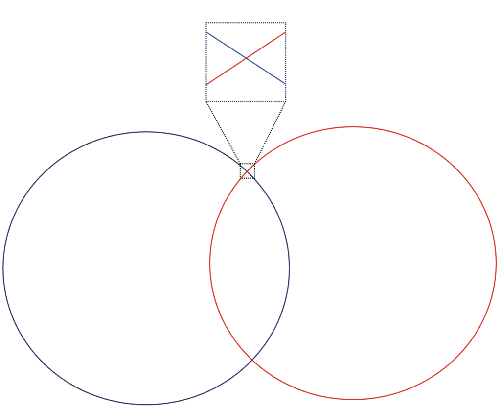
In practice, at least two sextant observations are required to obtain at least two position lines. Your ship’s position is then at the intersection of the lines obtained. In the image above, the intersection of the two position circles would give the ship’s position.
In the section on the theory of celestial navigation, we discussed the fact that, at the scale of nautical charts, the circles of position are so large that only segments of them can be seen.
Another consequence is that it is impossible to plot the GP of a celestial body on the chart showing the ship’s position. For example, if we are 3,600 nautical miles from the GP of a celestial body and the scale of the chart for our region covers a rectangle of approximately 200 nautical miles by 100 nautical miles, we can immediately see that we cannot have both the GP of the celestial body and its circumference (our position) on the same chart! The base is outside the chart. We therefore need a practical approach that allows us to draw lines to scale on the charts.
Azimuth, distance and line of position
Instead of drawing a position circle, we approximate it with a line representing the portion of the position circle on the map. To position this line on the map, we need its bearing (angle) and a point through which it passes.
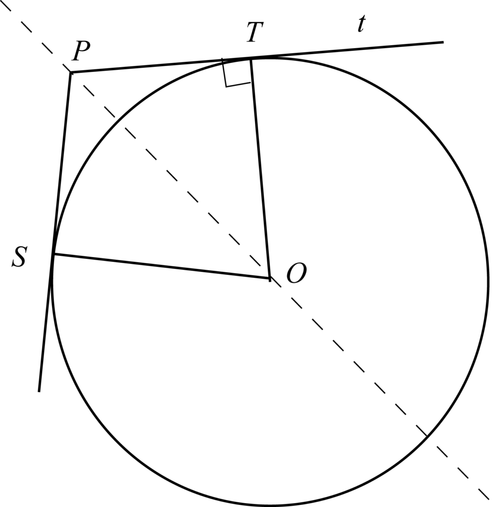
The bearing of the line of position is obtained by noting that any line approximating a part of a circle is tangent to the radius of the circle. In the image below, the line PTt is perpendicular to the radius TO.
Later, we will see how to perform the calculations to determine the direction of the GP of the celestial body, i.e. the direction pointing towards the centre of the circle. This direction is called the azimuth and is denoted Z_n. We can thus find the bearing of the position line by recalling that it is perpendicular (at 90°) to the azimuth.
The point through which the position line passes is obtained by calculating a distance from an estimated position. This distance will be either in the direction of the azimuth or in the opposite direction (Z_n or Z_n \pm 180°).
Combined, this information allows us to plot the position line.
An example
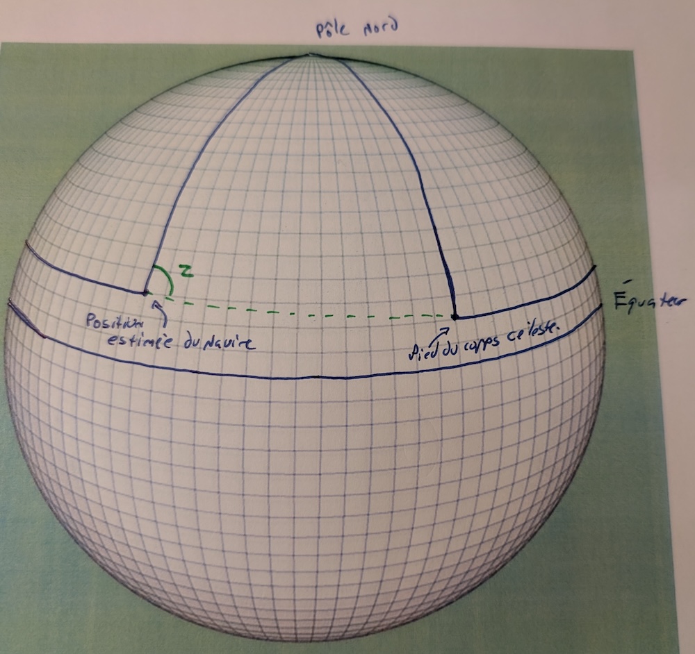
If we know the azimuth and the distance to a known point, we then have everything we need to draw a position line. To see this, let’s imagine we obtain the following information from our calculations:
- The azimuth of the GP of a celestial body is due south (180°);
- The position line is 15 nautical miles from our estimated position 10°N, 045°W;
- The distance is in the direction away from the GP of the celestial body.
Because the position line is perpendicular to the azimuth, we can deduce that it will lie in the direction of the bearing 270° (180° 90°), i.e. a line along the east-west axis. Because the line is further from the GP of the celestial body and the celestial body is due south, we also know that the position line is at the point 10° 15’N, 045°W, as one nautical mile equals one minute of latitude. Thus, the position line is an east-west line passing through the position 10° 15’N, 045°W.
In practice, this information is used to plot position lines on a chart.
Information required to plot a position
Four pieces of information are therefore required to plot a position:
- An estimate of our position, i.e. a position estimate.
- The azimuth of the GP of the celestial body (Z_n).
- The distance between the line of position and the estimated position.
- In which direction does the distance from the position line lie: towards the celestial body or away from it.
The estimated position is obtained by dead reckoning. This is preparatory work that must be carried out using standard navigation data: speed, course and drift. The more accurate this estimated position is, the more accurate our position derived from our calculations will also be.
The azimuth is obtained through spherical triangulation. This part is new, covered below, and requires either the use of reduction tables or trigonometric formulas.
The distance is estimated by comparing the corrected sextant reading (known as the observed height and denoted H_o) and the theoretical reading at the estimated position (called the calculated height and denoted H_c). The calculated height is obtained either by using reduction tables or by using trigonometric formulas. Both approaches are covered in this text. The observed height is obtained from the sextant reading to which corrections are applied and is the subject of an entire chapter.
We shall begin by covering the basics necessary to understand spherical triangles. Next, we shall show the two spherical trigonometry formulas for finding Z_n and H_c. Finally, we will show how to work with reduction tables. The first approach is more suitable for maths enthusiasts. The second is more suitable for those who find data tables easier to use than trigonometric equations. To each their own!
Introduction to spherical triangles
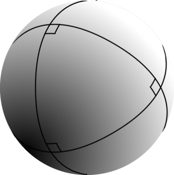
A spherical triangle is a triangle drawn on a sphere. The properties of spherical triangles differ from those of an ordinary (or ‘planar’) triangle. For example, the sum of the angles in an ordinary triangle is always equal to 180°. In a spherical triangle, the sum of the angles can be greater than 180°.
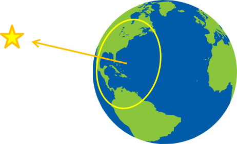
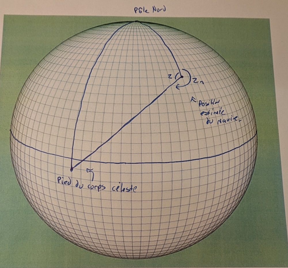
On Earth, we can imagine a triangle starting at the North Pole, travelling to the equator, following the equator for 5,400 nautical miles and then returning to the North Pole (image on the left). The sum of the angles of this spherical triangle is exactly 270°!
Because the geometry of spherical triangles differs from that of ordinary triangles, the formulas used to calculate side lengths and angles are not the same.
The four spherical triangles of celestial navigation
In celestial navigation, we are concerned with four categories of spherical triangles. They lie on the Earth’s sphere. These triangles are formed by the estimated position of the ship, the GP of the celestial body and one of the two Earth’s poles (either the North Pole or the South Pole). The pole chosen is always on the same side as the latitude of the ship’s estimated position.
The key properties that distinguish the types of triangles are whether the latitude of the estimated position is north or south, and whether a specific angle is greater than 180° or not. These conditions result in four categories of triangles.
The local hour angle (LHA)
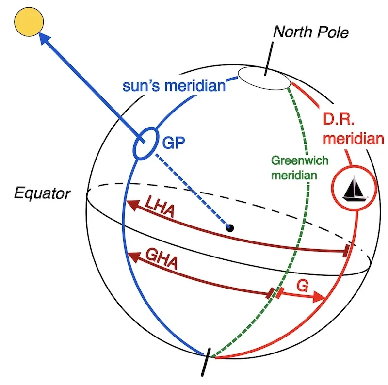
The angle relevant for the calculation is called the local hour angle (denoted LHA). The LHA is the angular hour difference between the estimated position of the ship and the GP of the celestial body. In other words, it is the difference between the GHA of the GP of the celestial body and the estimated longitude of the ship.
The LHA is measured from the ship’s estimated position and is always positive. In particular, when the GHA of the celestial body’s GP is less than the ship’s position, the difference will be negative. One must then add 360° to obtain a positive LHA.
Four triangles, four formulas
Each category of triangle requires a different calculation. Reduction tables or, alternatively, spherical trigonometry formulas will give us an angular difference denoted by Z. Then, depending on the nature of the spherical triangle, a different formula will be used to obtain the azimuth (Z_n) from Z. If you have understood the correspondence between the triangle and the formulas below, you will understand this section. The formulas are summarised in the table below.
| LHA < 180° | LHA > 180° | |
| Estimated latitude north. | Z_n = 360° - Z | Z_n = Z |
| Estimated latitude to the south. | Z_n = 180° Z | Z_n = 180° - Z |
To check your calculations, it is a good idea to understand why these formulas change depending on the triangle. The images and accompanying text below are intended to help you understand this.
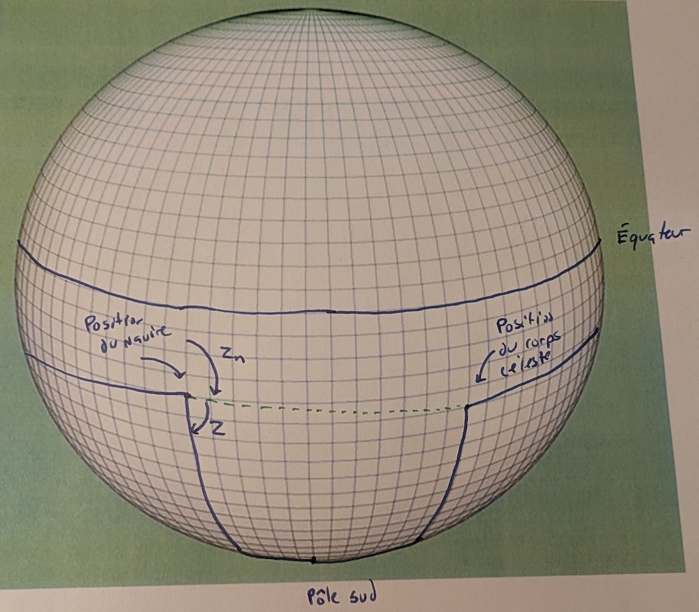
Spherical triangle #1
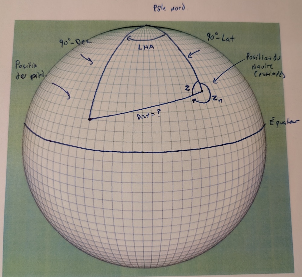
The first type of spherical triangle is illustrated in the image above. Note that the latitude of the estimated position and the declination of the celestial body’s GP are both in the Northern Hemisphere. Furthermore, the LHA is less than 180°, as all sides of the triangle are visible in the image.
If we focus on the ship’s position in the image, we see that the spherical trigonometry calculation Z and the azimuth Z_n add up to 360°. The image thus allows us to understand that if the latitude is north and the LHA is less than 180°, the azimuth is obtained using the formula:
Z_n = 360° - Z.
Spherical triangle #2
The second type of spherical triangle is such that the estimated position of the ship is in the southern hemisphere. Furthermore, the LHA is less than 180°, as all sides of the triangle can be seen in the image.
In this case, the image allows us to see that the azimuth Z_n is the sum of 180° and the angle Z:
Z_n = 180° Z.
Spherical triangle #3
In the third case, the estimated position of the vessel is in the Northern Hemisphere. However, the local hour angle (LHA) is greater than 180°. This can be seen in the image by the fact that one side of the triangle (in blue) is hidden because it passes to the other side of the sphere.
In this case, the spherical triangle calculations are performed using the angles of the complementary triangle (one side of which is shown in green dotted lines in the image). The calculated value of Z for this complementary triangle then corresponds directly to the azimuth.
Thus, if the LHA > 180° and the latitude is north:
Z_n = Z.
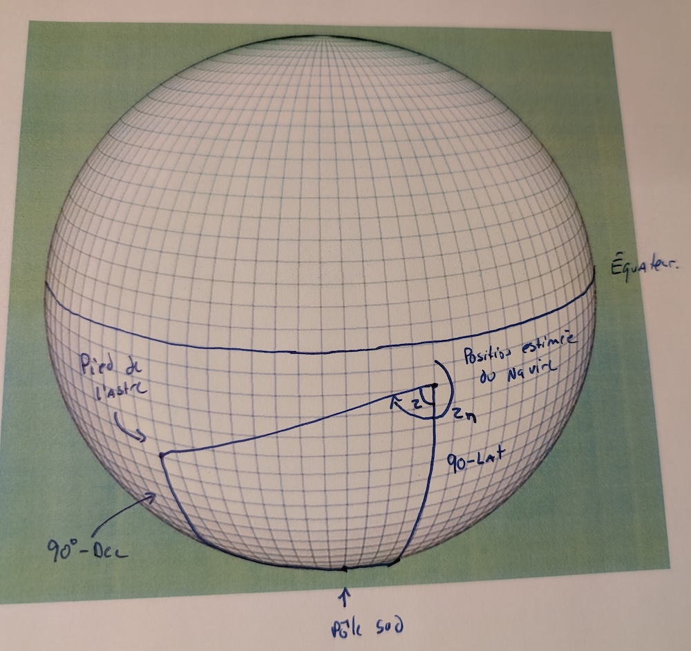
Spherical triangle #4
The fourth spherical triangle is such that the estimated position of the ship and the GP of the celestial body are in the southern hemisphere. Furthermore, the local hour angle (LHA) is greater than 180°, as one of the sides is behind the image.
In this case, the calculation of angle Z is performed on the complementary triangle (one side of which is shown as a green dotted line). The relationship between Z and the azimuth (Z_n) is then given by:
Z_n = 180° - Z.
Calculated height and Z using spherical trigonometry
If you are familiar with trigonometry, obtaining the calculated height H_c and the angle Z of each spherical triangle is obtained using the two formulas below:
\begin{align}
H_c&=\sin^{-1}\left[\sin(Dec)\sin(Lat) \cos(Lat)\cos(Dec)\cos(LHA)\right],\\
Z &=\cos^{-1}\left[\frac{ \sin(Dec) - \sin(Lat)\sin(H_c)}{\cos(Lat)\cos(H_c)}\right],
\end{align}
where Dec is the declination of the celestial body, Lat is our estimated latitude and LHA is the local hour angle. These formulas are an application of the law of cosines for spherical triangles.
It should be noted that the second formula requires the value from the first formula to be applied. They must therefore be calculated in order. It should also be noted that if the declination or latitude is in the southern hemisphere, a negative value must be used (e.g. 10° S = -10 in the formula).
In practice, simply enter the required values into a calculator, taking care to work in degrees. Most calculators accept arguments based on the decimal system. You must therefore convert the coordinates from the degree/minute/second format to the degree format with decimals (e.g. 10° 30′ = 10.5°). (It is also possible to work in radians, but the correction formulas must be adapted by replacing 180° with \frac{\pi}{2}, etc.).
For those interested, there is a good YouTube video on the derivation of these equations. For the purposes of astronomical navigation, one only needs to know how to use the equations.
Calculated altitude and Z using a reduction table
Reduction tables are the paper equivalent of a calculator. They are tables that do the calculations for us. For a given estimated latitude, a given LHA and a given declination, the tables will provide us with the calculated altitude H_c and the azimuth Z_n. The advantage is that no calculator (and no trigonometry) is required. However, the reduction tables run to over 1,000 pages and require some adaptation.
Adaptations
To reduce the size of the reduction tables, only whole degrees of latitude are given. Similarly, only whole degrees of LHA are recorded. Consequently, you must adjust your estimated position in two ways:
- Our estimated latitude must be the nearest whole degree;
- Our longitude must be such that the LHA is an integer. In other words, the difference between the GHA at the GP of the celestial body and our estimated longitude must be a whole degree.
These adjustments are irrelevant for determining the actual position, as we recall that the actual position is obtained relative to the estimated position. As long as the latter is not too far off, the approximation of circular segments by straight lines will be accurate. By staying at the nearest degree of latitude and choosing the longitude so that the LHA is an integer, the differences have little impact.
The pages of the reduction tables are also organised according to whether the latitude of the estimated position is in the same hemisphere as the declination or not. In the almanac, the word ‘name’ is used to indicate whether the declination/latitude is in the North or South. If the declination and latitude are of the same name, this means they are both in the same hemisphere (either North or South). If they are of contrary names, this means one is in the northern hemisphere and the other is in the southern hemisphere.
The image below shows two scenarios. The first image shows a case where the latitude and declination have the same sign. The image shows a declination and an estimated position latitude in the north. The second shows a case where the declination is in the south whilst the latitude is in the north. In this case, they have opposite signs.
There are other possible cases. These are summarised in the table below.
| Latitude in the north | Latitude in the south | |
| Declination North | Same name | Contrary name |
| Declination South | Contrary name | Same name |
Identify the appropriate page in the reduction tables
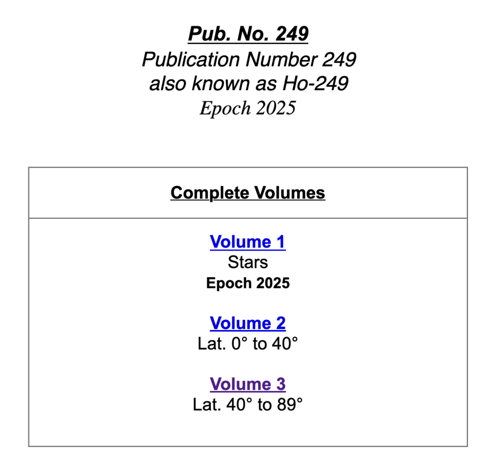
The reduction tables are presented in three volumes. Volumes two and three split the latitudes in two, notably to avoid having to carry too many pages on board one’s ship. One must therefore select the volume corresponding to the area in which one intends to sail.
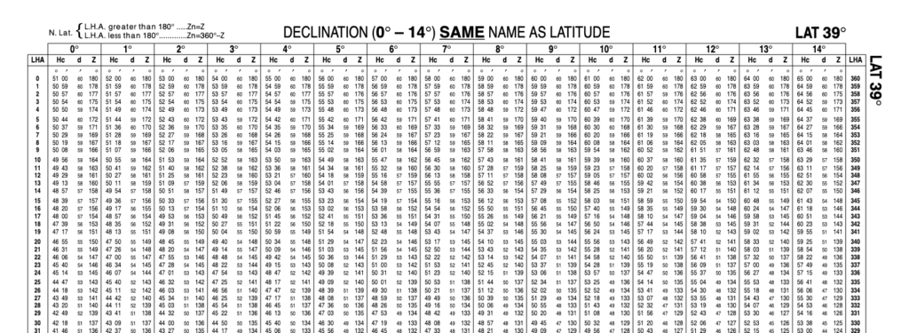
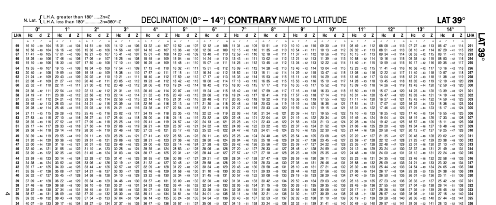
Each page is then organised according to latitude, a range of declinations and the name of the spherical triangle (SAME or CONTRARY). The image above shows the page for latitude 39°, declinations between 0° and 14° (columns) and a declination and latitude of the same name (SAME). The LHA is then provided for each row. By locating the intersection of a column and a row, one obtains the calculated height values (H_c) and the Z-angle. For example, we can see that for a declination of 6° and an LHA of 21°, H_c is 55° 56′ and Z = 145°.
Care must be taken with all the information in the reduction tables. Below, the image shows an extract from the table for a latitude of 39°, a declination range between 0 and 14°, and for a declination and latitude of opposite signs (CONTRARY). The two tables are almost identical! However, it can be noted that for a declination of 6° and an LHA of 21°, H_c is 40° 59′ and Z = 152°. It is a common mistake to use the wrong table. Therefore, it is good practice to check the table information twice before proceeding.
Once the adjustments have been made, finding the calculated height and the Z angle is simply a matter of consulting a table. The table is 1000 pages long, so you need to search through the volumes a little to find the right page.
Because the reduction tables require a modified estimated position, you must retain this modified position for subsequent calculations, as the distance and azimuth are based on this position.
Calculating the distance to the estimated position
Spherical triangulation calculations give us the calculated height H_c at this position. The sextant reading H_o gives the true distance to our true position. The difference between the two (H_c - H_o) gives us the distance in degrees and minutes. As one nautical mile corresponds to one minute of arc, we can convert this difference into distance to obtain the distance between the ship’s actual position and the observed position.
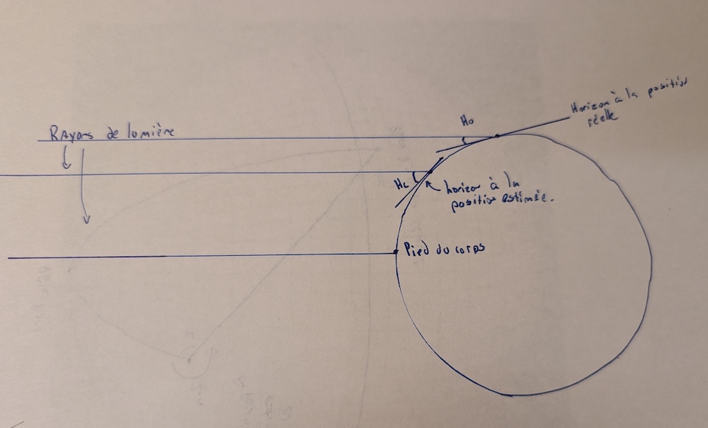
If the observed deviation H_c - H_o is positive, this means that the observed altitude is smaller than the calculated altitude. Consequently, we must move away from the GP of the celestial body. The diagram above illustrates this scenario. When the observed angle between the horizon and the rays of light from the celestial body is smaller than the calculated angle, this means that the position angle is greater.
If, on the other hand, the difference is negative, this means that the observed altitude is greater than the calculated altitude and one must move closer to the base of the celestial body. We can draw the same diagram as in the previous case, but with the positions reversed H_c and H_o. The analysis of the diagram remains the same.
Conclusion: procedural summary
It is a good idea to produce a procedural summary before moving on to the practical examples.
Key concepts:
- Reducing involves converting a sextant reading into a position line. To do this, you need an estimated position and the GP of the celestial body.
- The reduction will give us the azimuth of the celestial body (its direction), the distance from the estimated position of the line of position, as well as the direction relative to the estimated position.
- With this information, we can then plot a position line on a map.
- With several position lines, one can find the intersection of the lines and establish a position line.
- A spherical navigation triangle comprises the ship’s estimated position, the GP of the celestial body and one of the two poles (North or South). It is the mathematics associated with spherical triangles that allows us to find the angle Z and the calculated altitude H_c.
- There are four types of spherical triangles, each with a specific formula for converting the angle Z into azimuth Z_n. You need to know how to apply these formulas.
- The distance from the position line is obtained by calculating the difference between the calculated height H_c and the height observed with the sextant H_o.
- If H_c>H_o, the distance is increasing from the GP of the celestial body.
- If H_c<H_o, the distance is decreasing from the GP of the celestial body.
The procedure for performing a reduction:
- Note the declination of the celestial body, the estimated position of the ship and the altitude of the celestial body.
- Note the name of the latitude and the GP of the celestial body.
- Depending on your mathematical ability or ability to read tables:
- Use the spherical trigonometry equations:
- Calculate the local hour angle (LHA).
- Apply the formulas to find H_c and Z.
- Use the reduction tables.
- Find the value of your estimated latitude, rounded to the nearest degree.
- Find the value of your estimated longitude such that your LHA is a whole number.
- Calculate the local hour angle from your modified longitude.
- Identify H_c and Z in the reduction tables.
- Use the spherical trigonometry equations:
- Identify the appropriate calculation to convert Z to Z_n.
- Calculate the distance H_c-H_o:
- If it is positive, the distance from the actual position is approaching the celestial body.
- If it is negative, the distance from the actual position is moving away.
The next two sections will apply the procedure using examples.
If you enjoyed this text, you can read more in the Learn section of this site.


9 Responses
[…] trigonometry. To understand how to complete these exercises, you will need to have read the text on reducing sextant observations or, more generally, the series of texts on celestial […]
[…] for identifying the foot of a celestial body. The following article explains the technique for finding the position line associated with the observed […]
[…] this text, this information is assumed to have been obtained from sight reduction calculations. The examples below provide this information. The text focuses on using this information to plot […]
[…] the section on reducing sextant observations, we saw that the position lines are always at 90° to the azimuth of the star’s foot. […]
[…] Determine the azimuth Z_n by calculating the bearing. […]
[…] equations to obtain the calculated altitude (H_c) and the azimuth of the star (Z_n). The conversion recipe from Z to Z_n is the same for the first two stars, but differs for the […]
[…] the sun’s right ascension and our position, plus 360°. Thus, our LHA is 355° 58.9′. Using spherical trigonometry equations, we obtain </x></x></x></x></x>H_c = 63° 26.3′ and Z= 171° […]
[…] sight reduction exercisesusing the Ho 249 reduction tables. Beforehand, you should read the text on sextant observation reduction or, more generally, the series of texts on celestial […]
[…] technique is the subject of an entire text. However, the idea is straightforward: once the sextant measurements have been established, these […]