This seventh article in the series on astronomical navigation focuses on plotting position lines. This is the easiest part – and usually the last – of a positioning exercise. To do this, you will of course need a specialised sheet of paper for your plots, a parallel ruler and a pencil.
As discussed in the article on required publications and equipment, the specialised paper can be found in the final pages of the online Almanac. It is not mandatory (and depends largely on the size of your chart table), but I prefer to print these sheets in 11″ x 17″ format.
Four pieces of information required to plot a course
At the plotting stage, your sextant observations and calculations will have enabled you to extract four key pieces of information to establish a position line on which your vessel is located:
- an approximate position obtained by dead reckoning;
- the bearing of the foot of the celestial body from the approximate position (noted Z_n);
- the distance of the actual position line from the approximate position (noted \Delta H);
- whether this distance is in the direction of the celestial body or in the opposite direction (distance as it approaches or recedes).
In practice, the information might look like this:
- Your approximate position is 47° 25’N / 60° 40’ W;
- The sun’s position is in the direction of 173° from the estimated position.
- The distance of the position line is 3.9 nautical miles from the estimated position.
- This distance is away from the celestial body.
In this text, this information is assumed to have been obtained from sight reduction calculations. The examples below provide this information. The text focuses on using this information to plot your position.
Procedure for plotting
With these four pieces of information, you have everything you need to plot a position line. Using specialised plotting sheets, simply:
- construct the appropriate longitude scale;
- place the estimated position on the chart;
- from the estimated position, plot the line of direction from the foot of the celestial body;
- measure the distance in the correct direction (approaching or receding);
- draw the position line perpendicular to the direction line, at the identified distance.
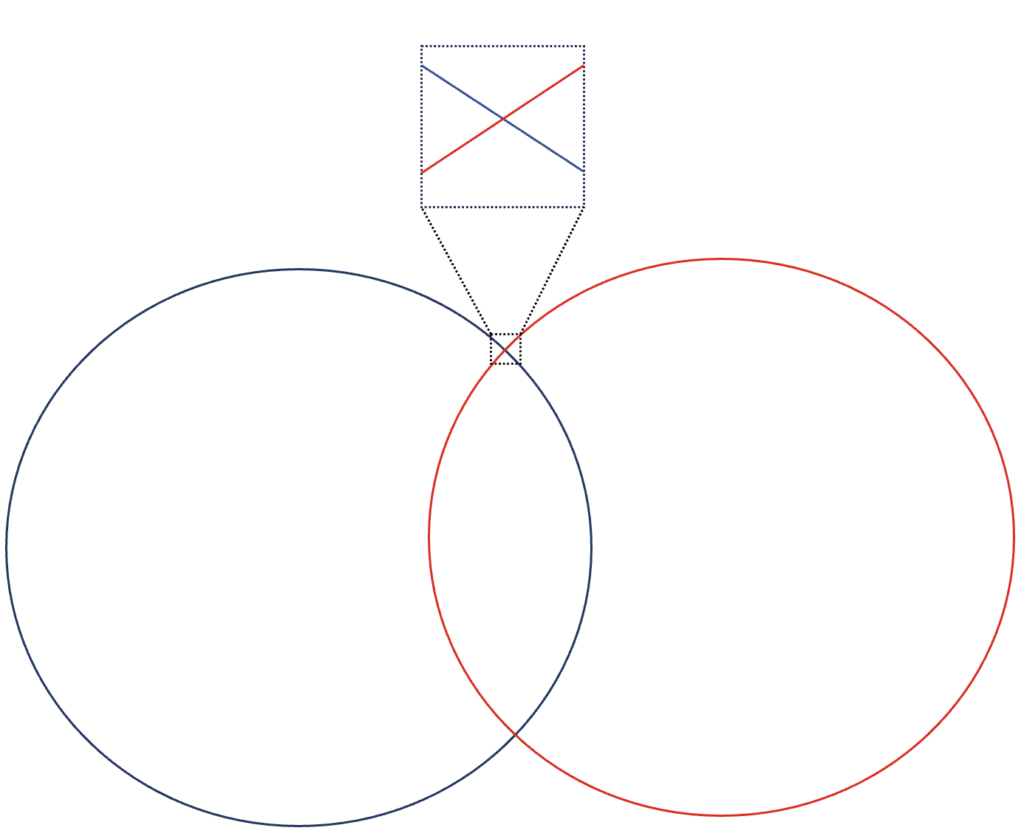
With more than one position line, the ship’s position can then be identified as the intersection of the position lines.
Plotting conventions
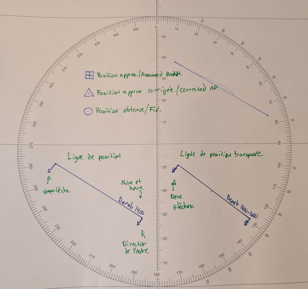
I use the Royal Yachting Association convention (above). This is mainly out of habit. As long as your charts are understood by those who will read them, it is perfectly acceptable to use a different convention. The RYA convention uses:
- A square for the estimated position (also used for a waypoint);
- A triangle for a corrected estimated position (where required);
- A circle for a confirmed position (a fix).
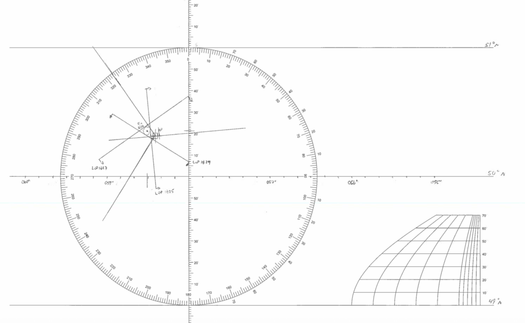
Position lines are annotated straight lines. Along the position line, usually in a place that does not interfere with reading the plots, the name of the celestial body used to obtain the position line, as well as the time of the sextant observation. In the image above, the (fictitious) sextant observation was made on the star Deneb at 1400.
Note also that position lines have arrows at their ends. These arrows indicate the direction in which the foot of the celestial body used lies. In the example shown above, the foot of Deneb would lie in the direction of 212°.
It may also be necessary to transpose a position line. In this case, the transposed line must be annotated with the name of the celestial body, the time of the original observation and the time of the transposition. The position line is then annotated with two arrows pointing in the direction of the celestial body’s meridian. In the example shown above, the transposed position line is linked to the star Deneb. The original observation was taken at 1400 and the time of transposition is 1600.
Constructing the scale of longitude
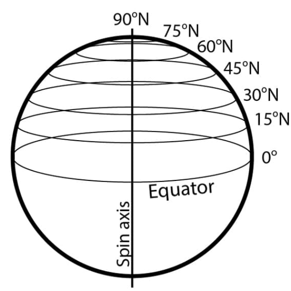
The scale of longitude varies with latitude. A one-degree difference in longitude does not represent the same distance depending on whether one is at the equator, at 45° latitude, or at the North Pole. This is because, depending on the latitude, the circles parallel to the equator change in size.
The image on the left illustrates this concept well. At the equator (0° latitude), the circumference is equal to the circumference of the Earth, so that one degree of angle is equal to 60 nautical miles. This is where the circle is largest. At 45° latitude, the circumference of the circle parallel to the equator is smaller. It is 70% of that at the equator, so one degree of angle corresponds to 42 nautical miles. At the North Pole (90°N latitude), the circumference of the circle parallel to the equator is zero! In short, the higher the latitude, the smaller the circles parallel to the equator will be.
The consequence is that the horizontal scales of maps vary with latitude. Our astronomical observation chart sheets are designed to work at any latitude. To do this, we must construct the longitude scale ourselves using the scale provided on the sheets.
Using the scale provided
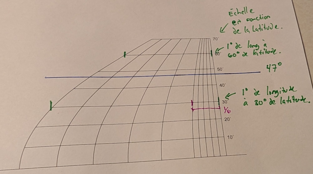
The scale at the bottom right of the astronomical plotting sheets allows you to find the appropriate scale based on the latitude of the observation. It shows the length of one degree of longitude as a function of latitude. At 30° longitude, the scale for one degree of longitude corresponds, on an 11 x 17 sheet, to approximately 6 centimetres. At 60° longitude, the scale for one degree of longitude, again on an 11 x 17 sheet, corresponds to approximately 3.5 centimetres.
Note that for each level, the scale is subdivided into six equal parts. As there are 60 minutes in a degree, each division corresponds to 10 minutes. Similarly, note that the last ten minutes are subdivided into five equal parts. Thus, each subdivision corresponds to two minutes. We can thus construct arbitrary lengths, in minutes, from the scale. For example, 40 minutes corresponds to 4 divisions on the scale.
In practice, we choose the latitude given by the approximate position. This is more than sufficient for our purposes. We must then construct the longitude scale on the main sheet by adding the degrees on either side.
Note that if the longitude is west, the scale increases by one degree as you move to the right. Conversely, if you are east, the longitude scale increases as you move to the left.
Constructing the latitude scale
The latitude scale is already marked, so all you need to do is identify the numerical values for each degree of latitude.
Note that the chart sheets have three horizontal lines. One is in the centre of the sheet and the other two are one degree of latitude higher and one degree lower than the centre line. To construct the scale, simply place the rounded latitude value of your estimated position to the right of the centre. Next, enter the subsequent values, bearing in mind that if you are in the northern latitudes, the scale increases as you move upwards. Conversely, if you are in the southern latitudes, the scale increases as you move downwards.
First example
Following your calculations based on your sextant readings, you have identified the following information regarding the Sun:
- Your approximate position is 47° 25’N / 60° 40’W at 1200 UTC-3.5;
- The Sun’s foot is in the direction of 173° from the estimated position.
- The distance to the position line is 3.9 nautical miles.
- The direction is away.
Plot the position line associated with this information.
Step 1: Construct the latitude and longitude scale
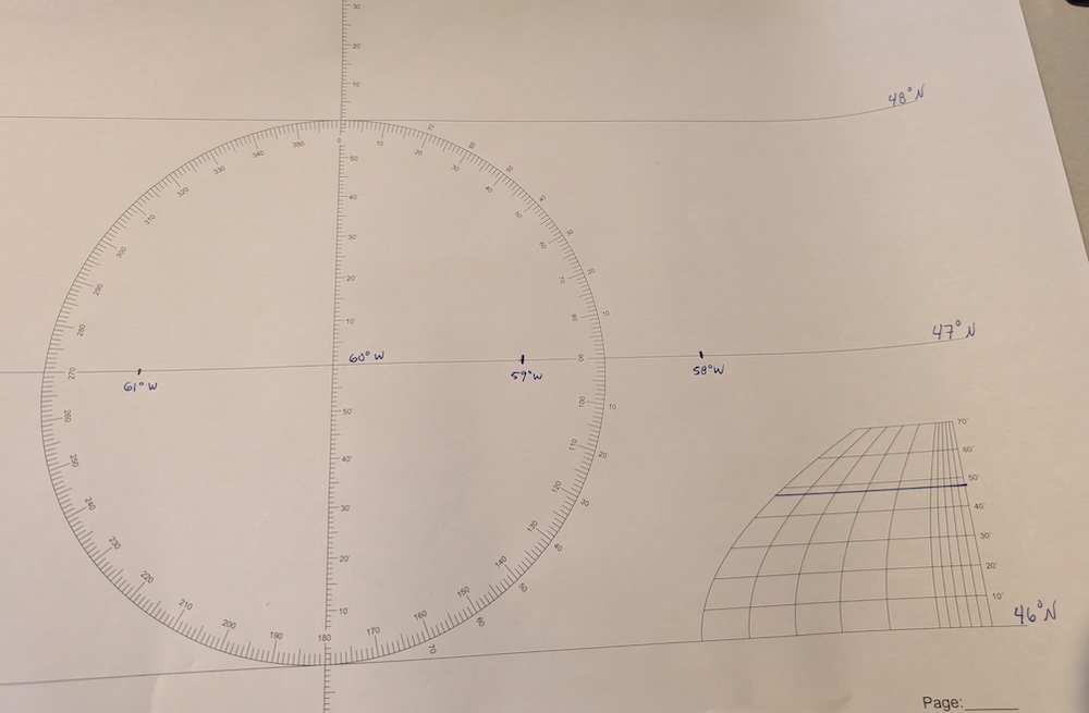
Our approximate position is at 47° north latitude. We therefore need to find the longitude scale for a latitude of 47°. The corresponding distance is shown in the image above. I therefore use this distance to construct the longitude scale. Because we are in western longitudes, the scale increases as we move to the right.
As for latitude, we are at approximately 47°N, so I use this as the central coordinate. Because we are in the northern hemisphere, the units increase as we move upwards. Thus, the top horizontal line corresponds to 48°N and the bottom horizontal line corresponds to 46°N.
The completed scale is shown in the image below. Note that I am using an ink pen to ensure it looks clear on screen. In practice, I would use a pencil for my annotations, so that I can erase any mistakes.
Step 2: plot the estimated position
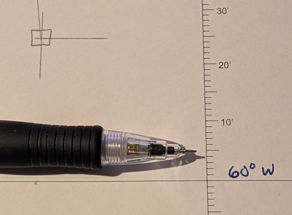
Our approximate position is 47° 25’N / 60° 40’W. Using the scale we have just drawn, we can plot this position.
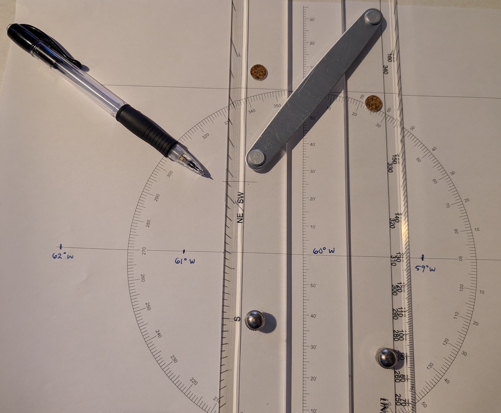
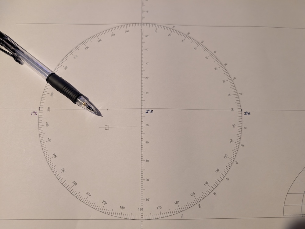
The best way to plot this position is to first draw the latitude, then use the longitude scale (bottom right) to identify the distance corresponding to the number of minutes. We can then use a ruler to transfer this distance to the appropriate latitude.
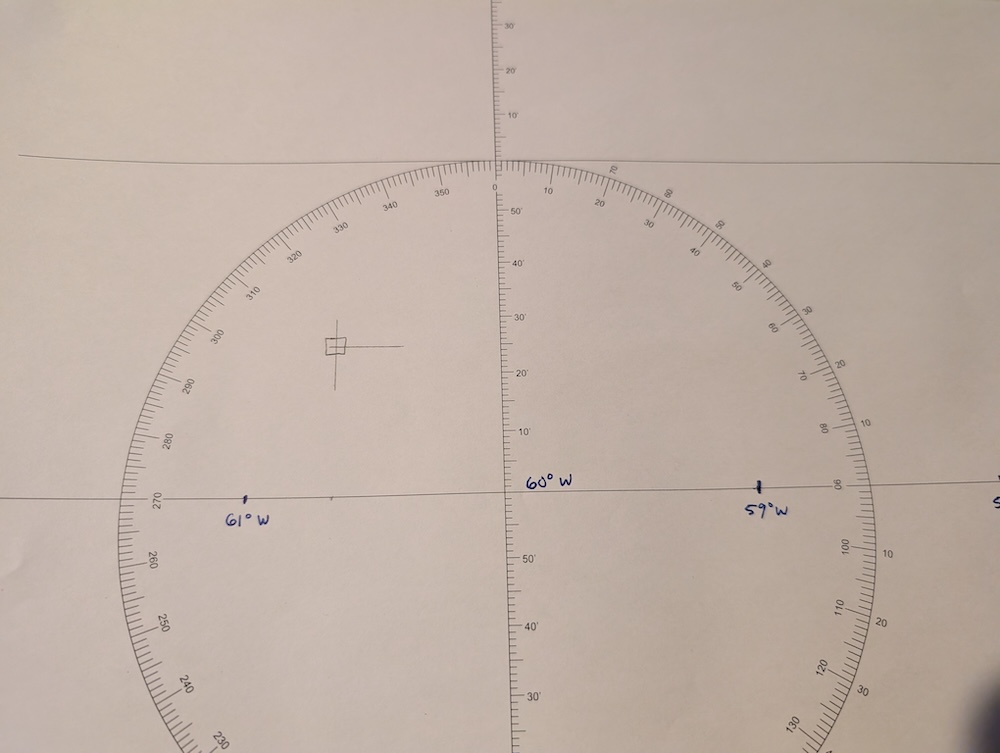
The first photo above illustrates the positioning technique. The second photo below shows the position plotted on the map.
Step 3: plot the direction of the foot of the body
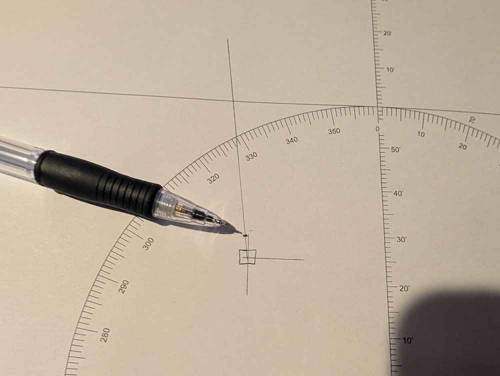
We know that the sun is in the direction of 173°, i.e. roughly south. We also know that the direction of the position line is 3.9 nautical miles away from the sun. We must therefore draw a line in the direction opposite to that of the sun (i.e. 173 + 180 = 353°). The idea is therefore to draw a straight line emanating from the approximate position and heading in the direction of 353°. If we had identified a distance approaching the sun, the line would have had to head in the direction of 173°.
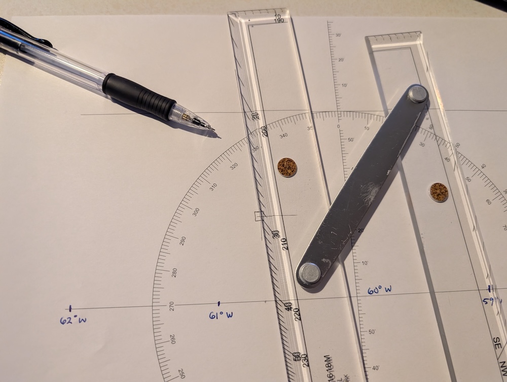
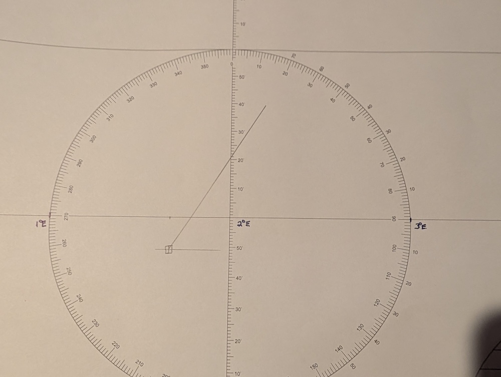
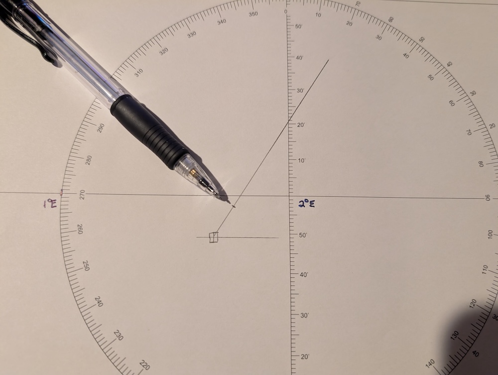
Below, I use a parallel ruler to identify the 353° direction, but you can also use a Breton protractor or a standard protractor. The first photo shows the parallel ruler set to 353° and passing through the approximate position. The second photo shows the line drawn.
Step 4: plot the distance
To plot the distance, measure 3.9 nautical miles on the latitude scale (vertical), bearing in mind that one minute corresponds to one nautical mile. Then transfer this distance along the line just drawn in step 3, in the appropriate direction.
In this example, the distance is 3.9 nautical miles away. You must therefore measure 3.9′ of distance on the horizontal axis (photo 1), then transfer it to the line away from the sun (photo 2).
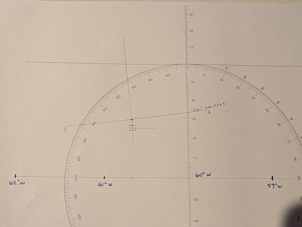
Step 5: draw (and label) the position line
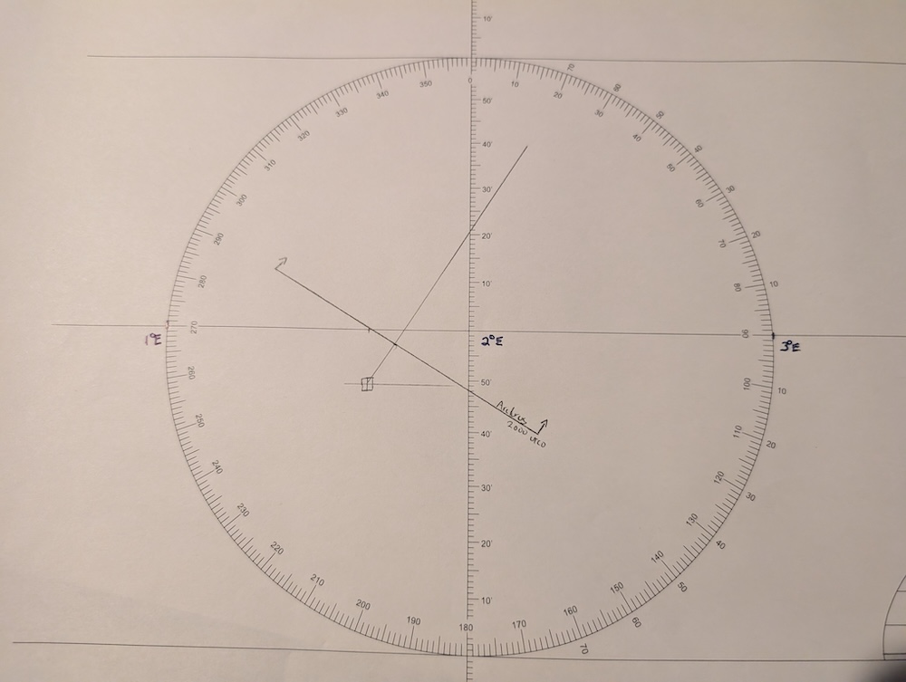
The final step is very simple: draw a line perpendicular to the line of distance identified in step 3, passing through the point of distance identified in step 4. This line of position corresponds to all points that are 3.9 nautical miles further from the Sun than the approximate position. If our sextant readings and the resulting calculations are correct, we know that the ship is on this position line at the time of the sextant reading.
The complete plot is shown in the image below. Obviously, at least two lines of position are required to determine the ship’s position.
Second example
At 2000 UTC – 0, you took a sextant reading of the star Arcturus.
- Your estimated position is 2° 11′ S, 001° 40′ E;
- Its bearing is 061°;
- The distance from the estimated position is 10 nautical miles.
- The position line is converging towards the star.
Draw the line showing your position.
Step 1: Construct the scales
We are in the Southern Hemisphere, in the eastern longitudes. Consequently, the latitude will increase as we move downwards and the longitude will increase as we move to the right. The central point of our plot will be 2°S 002°E. The photo below shows the appropriate scale.
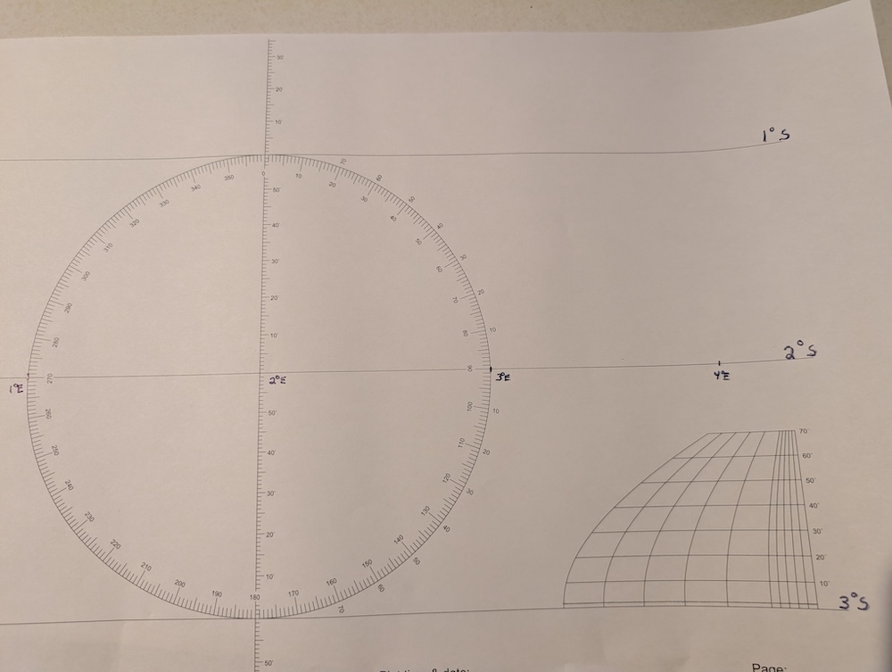
Step 2: Plotting the estimated position
The estimated position is shown in the image below. The only important detail to note in this plot is that, because the scales are reversed, you must pay attention to the directions to take. To increase the latitude by 11′, you must move down 11′ on the vertical scale. To increase the longitude, you must move to the left. The approximate position is illustrated in the photo below.
Step 3: Plot the direction of the foot of the body
In this example, you need to approximate the line of position of the star’s foot. You must therefore draw a straight line starting from the estimated position and extending in the direction of the star’s foot, i.e. at 061°. The line is shown below.
Step 4: Transfer the distance in the direction of the body’s foot
Here, we need to transfer a distance of 10 nautical miles. Read this distance on the vertical axis of our chart and transfer it along the straight line indicating the direction of the body’s foot. The photo above illustrates the transferred distance.
Step 5: Draw the position line
The position line is the line perpendicular to the line of direction of the body’s foot and passing through the distance identified in step 4. It is shown in the photo below. The vessel is located somewhere on this position line.
Third example
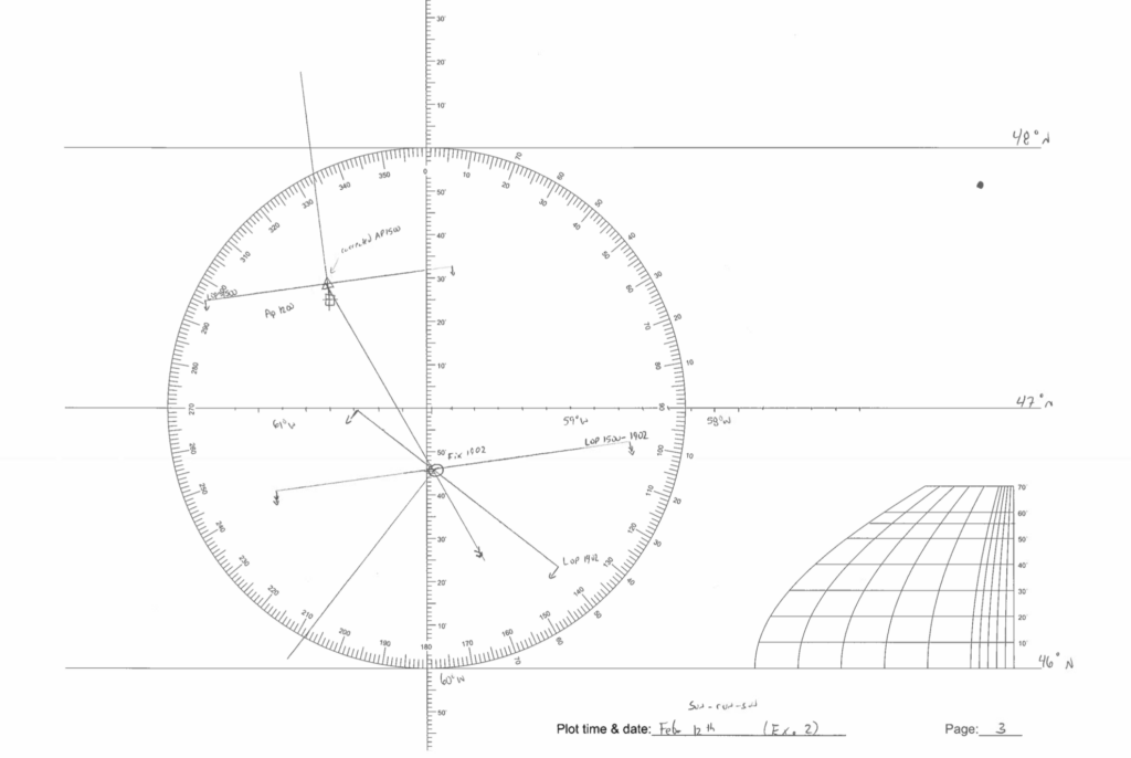
At an estimated position of 50° 19’N / 058° 24’W at 1830 UTC-3.5, you take sextant observations of the three stars Pollux, Rigel and Hamal. The details of each observation are shown below.
Identify the three associated position lines, as well as your position derived from the three sightings.
| Star | Pollux | Rigel | Hamal |
| Direction of the star’s foot (Z) | 85° | 145° | 211° |
| Distance from the position line | 3.0 min | 5.9 nm | 2.0 mn. |
| Approaching or moving away? | Moving away. | Moving away. | Getting closer. |
Solution
This time, there are three lines of position to plot. You must therefore repeat the plotting steps three times. The example is longer, but reflects the work involved in actual sextant observations. At least two, and usually three, lines of position are required to determine a ship’s position.
As in coastal navigation, the ship’s position will lie within the ‘position triangle’ corresponding to the intersection of the three lines of position. The complete solution is shown in the image below.
Conclusion
It is worth returning to our theory of celestial navigation. The ‘lines of position’ we have drawn are in fact approximations of circles of position around the foot of a celestial body. Because we are working with segments that are so small, they appear, for all practical purposes, to be straight lines.
These circles of position are derived from observations taken with a sextant. Using calculations set out in other texts, one can determine the direction of the celestial body’s meridian and the distance to the approximate position.
To break the subject down into different sections. This text focuses solely on the plots and on charts specialised for astronomical navigation. One must read the other texts to be able to understand how to calculate them.
Once the method is understood, it is simply a matter of repetition to obtain several lines of position. The ship’s position can then be determined at the intersection of these lines.
Did you enjoy this text? You can read more in the Learn section of this site.
1 Response
[…] In practice, this information is used to plot position lines on a chart. […]